Contents
NMDS Analysis
NMDS was calculated with both built-in Matlab function 'mdscale' and the Fathom toolkit function 'F_nmds.' (Jones 2015). Similar results were obtained with both methods and we used 'mdscale' for all downstream analysis.
% Clear enviornment and read in data
clear all; close all; clc;
cd '/Volumes/GoogleDrive/My Drive/Projects/Jesusthebotanist.github.io';
floralData = readtable('assets/code/scent/compounds.csv');

% Move to the FathomToolBox folder to call relavant functions.
cd ..
cd '/Volumes/GoogleDrive/My Drive/Projects/Jesusthebotanist.github.io/assets/code/scent/FathomToolBox/'


% Extract only scent data
floralScent = floralData(:,8:end);
floralScent = table2array(floralScent).';

% Calculate Bray-Curtis distance with Fathom Package
F_dissimilaritiesBC = f_braycurtis(floralScent);

% 2-axis nMDS with Matlab 'mdscale'
[F_Y,F_stress,F_disparities] = mdscale(F_dissimilaritiesBC,2,...
    'criterion','stress','Start','random','Replicates',500);

% 2-axis NMDS with Fathom Package 'f_nmds'
F_Fathom_nmds = f_nmds(F_dissimilaritiesBC,2);

% Compare Stress Value Output of Floral Data Between Matlab and
% Fathom Functions
disp ({'Matlab mdscale function 2 Axis Floral stress value =', F_stress});
disp ({'Fathom f_nmds function 2 Axis Floral stress value =',...
        F_Fathom_nmds.stress});
Warning: Variable names were modified to make them valid MATLAB identifiers.

---------------------------------------------------------
Selecting min STRESS from 10 random start configurations:
---------------------------------------------------------
29 iterations, Final stress criterion = 0.241458
29 iterations, Final stress criterion = 0.24884
40 iterations, Final stress criterion = 0.189437
68 iterations, Final stress criterion = 0.190346
30 iterations, Final stress criterion = 0.193859
55 iterations, Final stress criterion = 0.182521
32 iterations, Final stress criterion = 0.190076
36 iterations, Final stress criterion = 0.19389
22 iterations, Final stress criterion = 0.18319
33 iterations, Final stress criterion = 0.193855

Best configuration has STRESS = 0.1825212
---------------------------------------------------------
    'Matlab mdscale function 2 Axis...'    [0.1825]

    'Fathom f_nmds function 2 Axis ...'    [0.1825]
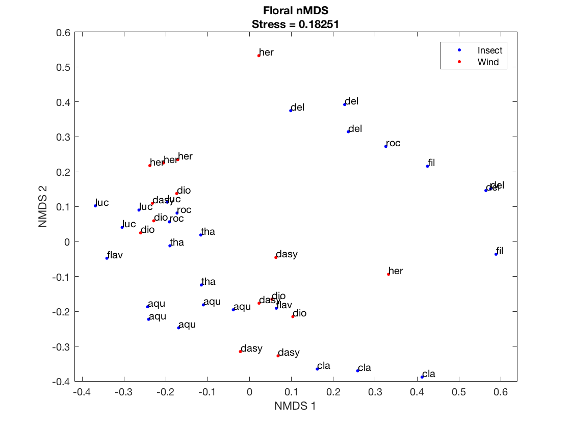
nMDS Plot
Plot a 2D nNMDS. These points are for Figure 2b
% 2-Axis nMDS plot with Pollination Syndrome Labels
figure(1);
    gscatter(F_Y(:,1),F_Y(:,2),...
        (table2array(floralData(:,{'Pollination_Syndrome'}))),'br','..>');
        legend('Insect','Wind');
        xlabel('NMDS 1');
        ylabel('NMDS 2');
        title({
             'Floral nMDS'
             ['Stress = ', num2str(F_stress)];
             });
    gname(table2array(floralData(:,{'Species_Name_Abbreviation'})));
1- Way ANOSIM
ANalysis Of SIMilarity (ANOSIM)is very similar to ANOVA, it is a method to determine if the means of grouping similar/different, however it is performed using the disimilarities rather than the raw data. We run ANOSIM grouping points by species (technical replicates) and by wind and insect pollinated taxa. We only find significance amongest species.
% ANOSIM - Group by Species
[F_r,F_p] = f_anosim(F_dissimilaritiesBC,...
            (table2array(floralData(:,{'F_name_number'}))),1,1000,1);

% ANOSIM - Group by Pollination syndrome
[FP_r, FP_p] = f_anosim(F_dissimilaritiesBC,...
               (table2array(floralData(:,{'Pollination_Syndrome'}))),...
               1,1000,1);
Permuting the data 999 times...

==================================================
         1-way ANOSIM RESULTS:
--------------------------------------------------
Sorted Groupings:
 1   1   1   2   2   2   3   3   4   4   4   4   4   5   5   5   5   5   6   6   6   6   7   7   8   8   8   8   8   9   9   9  10  10  10  10  10  11  11  11  11  11

Global Test:
  R = 0.5377  p = 0.0010 (1000 of 2722995984137736495806098899535396864 possible perms)

Pair-Wise Tests:
  1  2: R = 1.0000  p = 0.1000 (10 of 10 possible perms)
  1  3: R = 1.0000  p = 0.1000 (10 of 10 possible perms)
  1  4: R = 0.7641  p = 0.0179 (56 of 56 possible perms)
  1  5: R = 1.0000  p = 0.0179 (56 of 56 possible perms)
  1  6: R = 1.0000  p = 0.0286 (35 of 35 possible perms)
  1  7: R = 0.7500  p = 0.1000 (10 of 10 possible perms)
  1  8: R = 0.5692  p = 0.0179 (56 of 56 possible perms)
  1  9: R = 0.8519  p = 0.1000 (10 of 10 possible perms)
  1  10: R = 0.9077  p = 0.0179 (56 of 56 possible perms)
  1  11: R = 0.8974  p = 0.0179 (56 of 56 possible perms)
  2  3: R = 1.0000  p = 0.1000 (10 of 10 possible perms)
  2  4: R = 0.0564  p = 0.2500 (56 of 56 possible perms)
  2  5: R = 0.7641  p = 0.0179 (56 of 56 possible perms)
  2  6: R = 0.7037  p = 0.0286 (35 of 35 possible perms)
  2  7: R = 0.5833  p = 0.1000 (10 of 10 possible perms)
  2  8: R = 0.2205  p = 0.1607 (56 of 56 possible perms)
  2  9: R = 0.1111  p = 0.3000 (10 of 10 possible perms)
  2  10: R = 0.7641  p = 0.0179 (56 of 56 possible perms)
  2  11: R = 0.1077  p = 0.3214 (56 of 56 possible perms)
  3  4: R = 1.0000  p = 0.0476 (21 of 21 possible perms)
  3  5: R = 1.0000  p = 0.0476 (21 of 21 possible perms)
  3  6: R = 1.0000  p = 0.0667 (15 of 15 possible perms)
  3  7: R = 1.0000  p = 0.3333 ( 3 of  3 possible perms)
  3  8: R = 0.9455  p = 0.0476 (21 of 21 possible perms)
  3  9: R = 0.6667  p = 0.2000 (10 of 10 possible perms)
  3  10: R = 0.5818  p = 0.0476 (21 of 21 possible perms)
  3  11: R = 0.6545  p = 0.0476 (21 of 21 possible perms)
  4  5: R = 0.3440  p = 0.0476 (126 of 126 possible perms)
  4  6: R = 0.1500  p = 0.1508 (126 of 126 possible perms)
  4  7: R = -0.0182  p = 0.4762 (21 of 21 possible perms)
  4  8: R = 0.0600  p = 0.2857 (126 of 126 possible perms)
  4  9: R = 0.2821  p = 0.0536 (56 of 56 possible perms)
  4  10: R = 0.8000  p = 0.0079 (126 of 126 possible perms)
  4  11: R = 0.0720  p = 0.2937 (126 of 126 possible perms)
  5  6: R = 0.9875  p = 0.0079 (126 of 126 possible perms)
  5  7: R = 0.6364  p = 0.0476 (21 of 21 possible perms)
  5  8: R = 0.3760  p = 0.0159 (126 of 126 possible perms)
  5  9: R = 0.7949  p = 0.0179 (56 of 56 possible perms)
  5  10: R = 0.9800  p = 0.0079 (126 of 126 possible perms)
  5  11: R = 0.4800  p = 0.0079 (126 of 126 possible perms)
  6  7: R = 0.7857  p = 0.0667 (15 of 15 possible perms)
  6  8: R = 0.5875  p = 0.0238 (126 of 126 possible perms)
  6  9: R = 0.3333  p = 0.0571 (35 of 35 possible perms)
  6  10: R = 0.8187  p = 0.0159 (126 of 126 possible perms)
  6  11: R = 0.2750  p = 0.0159 (126 of 126 possible perms)
  7  8: R = 0.2000  p = 0.1429 (21 of 21 possible perms)
  7  9: R = -0.0000  p = 0.5000 (10 of 10 possible perms)
  7  10: R = 0.8364  p = 0.0476 (21 of 21 possible perms)
  7  11: R = -0.0364  p = 0.4762 (21 of 21 possible perms)
  8  9: R = 0.3128  p = 0.0893 (56 of 56 possible perms)
  8  10: R = 0.7760  p = 0.0079 (126 of 126 possible perms)
  8  11: R = 0.4080  p = 0.0397 (126 of 126 possible perms)
  9  10: R = 0.3641  p = 0.0893 (56 of 56 possible perms)
  9  11: R = 0.1692  p = 0.1786 (56 of 56 possible perms)
  10  11: R = 0.5400  p = 0.0238 (126 of 126 possible perms)

==================================================

Permuting the data 999 times...

==================================================
         1-way ANOSIM RESULTS:
--------------------------------------------------
Sorted Groupings:
 1  1  1  1  1  1  1  1  1  1  1  1  1  1  1  1  1  1  1  1  1  1  1  1  1  1  1  2  2  2  2  2  2  2  2  2  2  2  2  2  2  2

Global Test:
  R = -0.0376  p = 0.2390 (1000 of 98672427616 possible perms)

Pair-Wise Tests:
  1  2: R = -0.0376  p = 0.7210 (1000 of 98672427616 possible perms)

==================================================
References
Jones DL. 2015. Fathom Toolbox for Matlab: software for multivariate ecological and oceanographic data analysis. College of Marine Science, University of South Florida, St. Petersburg, FL, USA. http://www.marine.usf.edu/user/djones/